Description.

The task of the Predictive Tire Health Monitoring System is to detect tire leakages as soon as possible, to identify the trend of the leakage, and possibly, to generate alarms when the pressure tends to fall down for example, when a tire is punctured. If the speed at which a tire loses its pressure does not exceed 1 bar/day, it is considered to be a slow leakage; if the speed exceeds 1 bar/day, a fast leakage is to be reported. The Predictive Tire Health Monitoring System is supposed to work in real time by accepting a stream of the tire pressure supplied with its time stamp.

Properties of the pressure signal being delivered.

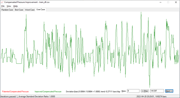
Pressure in vehicle tires is measured with certain errors; below is a typical curve of so-called, "compensated pressure" depending on time. Presence of such errors makes it difficult to spot a trend as the pressure constantly jumps up and down even in an absolutely healthy/non-punctured tire:

Picture 1. Typical behaviour of tire pressure upon time.

As it has been observed, the distribution of tire pressure being measured (the green curve) is close to be Gaussian (the grey curve):

Picture 2. Typical distribution of tire pressure.

Let us detect possible leakages by identifying a trend at which the tire compensated pressure gets changed. The best mathematical approach for detecting the trend is composing a maximum likelihood equation (or, equations) and calculating its (their) values at the actual observation points. The higher the value of such an equation at the actual data, the more likely that particular equation (or, the equation parameter for parameterized equation) reflects the trend.

Let us compose the maximum likelihood equation for our case given that the distribution density is Gaussian. Let us assume that the trend is described by a linear equation y_i = a · t_i + b. A negative value of "a" means that the tire loses its pressure whilst a positive one reflects the fact that the tire is inflated again, and that its normal pressure has been restored.

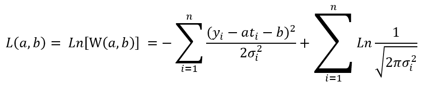
 The maximum likelihood equation:

where: t _i - time of measurement; y_i - pressure measured at the time t_i ; σ_i² - variance of pressure measurements at the time t_i 

Equation 1.

Note, that W(a, b) and its natural logarithm reach their maximums exactly at the same point, which allows us to replace W(a, b) with its natural logarithm.

The logarithmic maximum likelihood equation:

Equation 2.

Equation 2 reaches its maximum at a point at which its partial derivatives by the equation parameters "a" and "b" are zeros.

Derivatives of the above log-likelihood function:

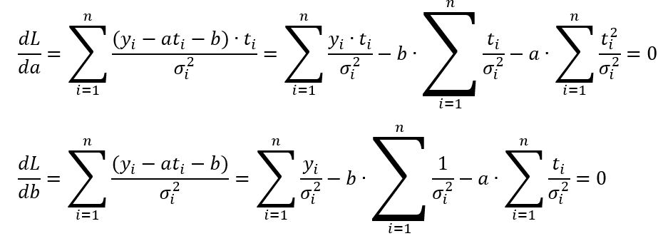
Equation 3.

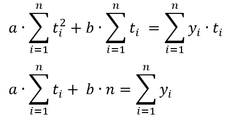
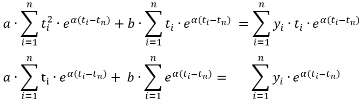
So, "a" and "b" are solutions of the following matrix equation:

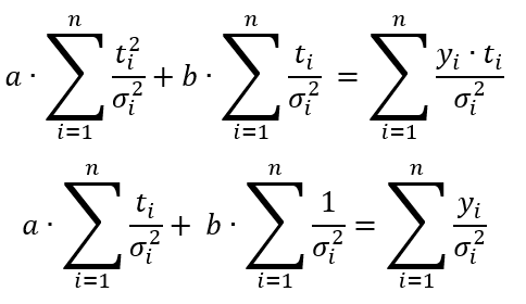
Equation 4.

Note, that if we assume that , then the deviations cancel each other, and the equations become fully identical to those for finding a line that minimizes the sum of the squares of the residuals at each individual time point:

Equation 5.

Now, old measurements should have a decreasing influence on the trend estimate, up to negligible. To reach this goal, assume that the standard deviation gets increased in the past in the geometric progression. In this case, the density of the Gaussian distribution tends to be flat, which makes the original maximum likelihood equation values be almost independent on the measurements preformed far in the past. To reach this goal, assume that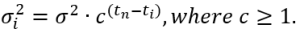

In this case, the equation for "a" and "b" becomes as follows:

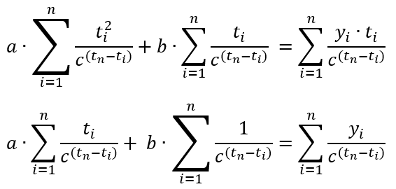
Equation 6.

Note, that the linear approximation (e.g., the trend, itself) y = a + b · t does not depend on the pressure variance σ²! Despite this, the variance of the trend does depend on the pressure variance.

Let us denote 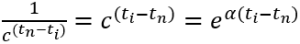, where α = ln(c):

Equation 7.

Note, that if α = 0 (e.g., c =1), Equation 7 becomes identical to Equation 5 above.

Let us call the value of α ≥ 0, the "memory coefficient". When α is zero, the system remembers all the data and identifies the trend based on the entire history available. However, as α gets increased, the system gives preference to the fresh/most recent data. Thus, the trend "y = a + b · t" is built on mostly the latest points {t_i, y_i}, which is just the goal. The more the memory coefficient, the faster the system forgets data in the past. Examples are provided below; see pictures 3 and 4 below.

Picture 3. A pressure trend without a memory coefficient.

Picture 4. A pressure trend with some positive memory coefficient.

Properties of trends.

Let us consider some properties of trends we've defined above.

1. The trend standard deviation is in direct proportion with the one of the pressure: "Dev(Trend) = a · Dev(P)", where a is some constant that depends on the variance memory coefficient.

Proof. Let vector x be a solution of the matrix equation  A·x = B, where B is some pre-defined vector. Let B' = λ·B. Then, obviously, x' = λ·x is a solution of the equation A·x' = B'. Now note, that the pressure in the equation 7 is present only in the right side, and that if we multiply all pressure values by some λ, then the right side of the equation will be just B' = λ·B. But, the variance Var(λ·B) = λ² ·Var(B) whilst the standard deviation, just λ, is in direct proportion with the pressure standard deviation. ■

This means that the only way to improve the trend precision is to improve precision of the measuring equipment.

2. Assume, you calculate some trend on a given number of payloads, e.g., the last 100 payloads. Assume also that a matrix for the previous say, 100 payloads has already been calculated. Is there any way to quickly re-calculate the matrix given that the very first payload disappears while the new one comes in?

The answer is, "yes, there is". Let us first, look at the equation 5, which is a simplified version of equation 7. Indeed, it is obvious that the new matrix coefficients will be as follows:

a) [New Σ t_i² ]= [Old Σ t_i²] + (t_n² - t₁²),

b) [New Σ t_i ]= [Old Σ t_i] + (t_n - t₁),  etc.

Very easy, isn't it? Indeed, but there appears another problem, namely: calculation errors accumulate! (t_n - t₁) and similar terms are actually, random variables, so when we add them each time a new payload comes, the overall error grows up! We've even been facing appearance of singular matrices in equation 7 from time to time, after which realized that trends with a zero memory coefficient aren's quite suitable for us. To let you better feel the deepness of the problem, run the following Python code, which iteratively adds 3 numbers to zero, than substracts the same numbers but in some random order, after which the original zero value constantly keeps on growing up:

import random

ITERATION_COUNT = 100000
S = 0
A = [0, 0, 0]
for iteration_number in range(ITERATION_COUNT):
    A[0] = random.randint(0, 256) / (256 + random.randint(0, 256))
    A[1] = random.randint(0, 256) / (256 + random.randint(0, 256))
    A[2] = random.randint(0, 256) / (256 + random.randint(0, 256))

    i = random.randint(0, 2)
    S += A[i]
    i = (i + 1) % 3
    S += A[i]
    i = (i + 1) % 3
    S += A[i]

    i = random.randint(0, 2)
    S -= A[i]
    i = (i - 1) % 3
    S -= A[i]
    i = (i - 1) % 3
    S -= A[i]
# for iteration_number

print(S)

3. The situation changes dramatically when we look at the equation 7, with some positive (non-zero) memory coefficient. To re-calculate/adjust the matrix coefficients, it is not required to deduct the very old points: they are already automatically "forgotten" (e.g., multiplied by zeros) by the very nature of trends with memory. So, trends of this sort do not need re-calculating the matrix coefficients from time to time, and do not require storing old points. Here's how formulas for adjusting the matrix coefficients when a new payload appears look like:

a) [New Σ t_i² ]= [Old Σ t_i²]·e^{α(t_n-t_n+1)} + t_n²,

b) [New Σ t_i ]= [Old Σ t_i]·e^{α(t_n-t_n+1)} + t_n , etc.

(you may prove the above formulas by yourself by applying the rule e^α+β= e^α·e^β)

Calculation errors in such equations get automatically multiplied by coefficients that are less than 1 and thus, they fully eliminate by approaching zero as new payloads appear.

Provided below is a sample code snippet which demonstrates how easily the trend matrix coefficients are adjusted upon appearance of a new payload:

class trend
    ...
    def add_payload(self, time: float, pressure: float) -> None:
        multiplier = exp(memory_coefficient * (previous_time - time))

        self.Sx2 = multiplier * self.Sx2 + time * time
        self.Sx  = multiplier * self.Sx  + time
        self.Sxy = multiplier * self.Sxy + time * pressure
        self.Sy  = multiplier * self.Sy  + pressure
        self.S0  = multiplier * self.S0  + 1
    # def add_payload()

4. Given, that old measurements have a decreasing influence on the trend estimate, we can calculate a point in the past, at which all data beyond that point have no influence on the trend at all. This will give us an upper estimate of the period of time, after which our Tire Health Monitoring System completely "forgets" old data. The following table provides such an estimation:

Table 1. Memory period and standard deviation of trends.

Summary.

1. Trends with memory require storing only 5 (five!) real numbers regardless of the number of payloads: 3 matrix coefficients of 4 (2 are identical) plus 2 in the free vector = 5.
2. Trends with memory can be quickly re-calculated when a new payload comes in.
3. Trends with memory are resistant to calculation and measurement errors.
4. Their standard deviation is proportional to the standard deviation of the pressure, itself.
5. If we substitute t for ṫ=λ·t, then the new trend becomes equal to å=a/λ. In other words, if the time gets stretched in the λ proportion, the updated trend gets divided by λ. To provide a proof, just substitute t for λ·t in the equations 7 and 5. ■
6. Regardless of the pressure standard deviation (e.g., regardless of the precision at which pressure gets measured), there is some memory coefficient, with which a corresponding trend signalizes pressure deflation at a required probability of possible error. Indeed, when the memory coefficient tends to zero, so does the trend deviation. ■
7. The response time (e.g. the amount of time that is required for the trend to detect a leakage after it starts) has a directly proportional relationship with the standard deviation of the pressure measurement. It means that the less accurate are the measurements, the longer it takes for the trend to detect a leak. Below is an estimation of the response time depending on the leakage speed. It can be improved by either/or sending payloads more frequently (once 5 minutes instead of each 15 minutes, for example), or/and by improving the pressure measurement precision.
8. Finally, note that in the above table: a) the result of the trend memory period and the trend standard deviation is a constant, b) the period is in the inversely proportional relationship with the memory coefficient, and c) the trend standard deviation is in the directly proportional relationship with the memory coefficient.

Table 2. The System Response Time estimation depending on the leakage speed.

Given all the above, it looks like trends with memory are exactly what we need to predict possible pressure deflations, aren't they. Let us use such trends in our Tire Health Monitoring System system, then. How? Let us calculate a series of trends for each tire, and if at least some trend value falls out from its confidence interval, consider a leakage to be detected. See also, the rule 68–95–99.7.

The programming realization of the leakage detection algorithm is described in more detail in the document "The LEDP Algorithm Description". Its characteristics such as, its robustness, performance, the false positive and the false negative probabilities shall be provided there. ("False positive" is an occurrence when the system erroneously reports a leakage whilst "false negative" is a case when the system does not notice a leakage even though the tire is punctured).

Appendix 1. How the system stops reporting a leak after it's gone.

When a leakage disappears (for example, when the puncture gets fixed and the tire inflated, again), the system remains reporting the leakage until the system makes sure that it has gone away indeed. The following formula approximates the number of payloads during which the system keeps on reporting a leakage (e.g., remaining payloads R) depending on the number of payloads within the leakage (L):

R = -0.0000271453062905218•L² + 0.0526910994830675•L + 95.0901489390417

Examples: R(2880) = 25 (slow leak); R(1440) = 95 (fast leak), ... R(132) = 75 (very fast leak).

Actually, the value of R depends on:

a) The entire pressure curve of the tire (e.g., on ALL previous payloads related to the tire within at least the latest 2 months)

b) All the payloads related to all the tires in a fleet as the system calculates and takes into account the variance with which pressure gets measured within all tires of the fleet.

So, the above formula provides a very rough estimation of the remaining number of payloads. It has been build under the following scenario: initially, a constant pressure of 10 bars with the standard deviation of 0.1 bar. Then, deflating till 5 bars at different speeds with a 5-minute interval payloads. Finally, restoring the original 10-bars pressure and counting the number of payloads during which the system still keeps on reporting a leakage (R).

Under other scenarios the above simplified formula is not applicable. For example, for a single short drop 10 bars → 0 bars → 10 bars, again, the system reports a leakage for several remaining payloads only (as a rule, just 3 extra payloads).

Appendix 2. Some knowledge consolidation tasks:

Task 1.  At the end of paragraph 3 there is a sample code snippet, in which the last statement is:

self.S0  = multiplier * self.S0  + 1

Does the value of "self.S0" have a limit as the add_payload() function gets called iteratively? Under what conditions does it have? If it does, what is the value of the limit?

Solution. It does when the payloads are obtained at exactly the same interval: 15 minutes, for example. In this case the value of "multiplier" is constant, which allows us to consider the  above statement as an equation. The solution of the equation is: S₀ = (1 - multiplier)^-1

Task 2.

Assume, you start obtaining tire pressure from multiple (hundreds of thousand of) wheels that have been equipped with the same pressure measuring hardware and therefore, all have the same measurement variance. However, the pressure, itself in each wheel is different, so the mathematical expectation of the tire pressure is individual for each wheel (and is unknown to you). Assume also, that each wheel reports its tire pressure once each 15 minutes. What would be your estimate of the tire pressure variance in: a) 15 minutes from starting obtaining the data? b) 30 minutes? c) one day, etc.? What would be precision of your solution?

Solution. Let us consider the random variables (P_i - P_i-1 ) for each wheel, which are just differences between neighbouring values of pressure from the same tire. All these differences have the zero mathematical expectation and the same variance, which is 2 * Var(P). So, in 15 minutes we are having hundreds of thousand of random variables with the same mean and variance. This task has a standard solution for finding the variance. Having solved it, the variance of the pressure, itself is one half of the variance of its neighbouring differences. ■

Task 3.

Assume, that a customer starts providing our Tire Health Monitoring System with payloads each 5 minutes instead of 15 minutes (e.g., three times faster). How exactly will this affect the System Response Time? What happens if we assume for a moment that payloads are being reported once a minute? You do not have to provide any mathematical proof just express your opinion, please. Thank you!

Solution. Trends behave like an estimation of the random variable average: when a number of points gets increased, the resulting estimation standard deviation gets decreased at a square of the number of points proportion. This means that if the density payloads increases in three times (once each 5 minutes instead of 15 minutes), the System Response Time gets decreased into √3 = 1.73 times. If the Tire Health Monitoring System gets provided with payloads once a minute, the System Response Time will decrease in √15 = 3.87 times.

Please, send your propositions to Sergey Kryloff by the e-mail sergeyk@soborka.net. The winner gets the prise! The prise remains at Sergey Kryloff's ownership as nobody has solved the tasks.